Which way would a drug have to push each LDL gene?
A complete Inflexa session on the GLGC LDL cholesterol GWAS: 44 million variant records with no LD reference panel available, every canonical target recovered with the correct direction of intervention including the two that run backwards, and a nearest-gene call that fails at the third-strongest signal in the genome.
GWAS Catalog GCST90239658, the European-ancestry stratum of the Global Lipids Genetics Consortium lipids meta-analysis (Graham et al., Nature 2021, PMID 34887591). LDL cholesterol, quantitative, N up to 1,320,016. One harmonised gzipped table of 44,246,098 variant records, autosomes only, GRCh38, 1.3 GB, plus a 1.7 MB tabix index. GWAS Catalog accession
GWAS summary statistics are the most generous public data in human genetics. No consent barrier, no genotypes to protect, no application to fill in. A well-powered lipids scan is a plain table you can download and read, and it is the closest thing target discovery has to a benchmark: everyone knows what the answer is supposed to look like, because statins and PCSK9 inhibitors already exist.
Which makes it a good place to ask a harder question than "what are the top hits". A hit names a region. A drug programme needs a gene and a direction, and the two are not equally easy to get from summary statistics. That gap is what this session is about.
Everything below is one session. The prompts are quoted exactly as they were typed, and the screenshots come from the run that produced the figures on this page.
- Direction survives the missing LD panel. Gene identity does not. All nine canonical LDL drug targets came back with the correct direction of intervention, while 369 of 396 loci were left with no gene evidence beyond proximity.
- Two of the nine run backwards, and one of them is the second-strongest signal in the genome. ABCG5/ABCG8 needs activation and LDLR needs augmentation, not inhibition. A pipeline that assumed "lipid gene, therefore inhibit" would have inverted both.
- Nearest-gene fails at rank 3. The chr1p13 locus is labelled PSRC1 by transcription start site and CELSR2 by gene body. The causal gene is SORT1, which is in the window and is named by neither metric. The two distance metrics also disagree with each other at 32.6% of all loci.
- ClinVar, filtered to lipid conditions, recovers four genes proximity missed: ANGPTL3, APOC3, LDLRAP1 and LIPA. Two of the four sit inside or overlapping a neighbouring gene, so no distance metric could have reached them.
- A genomic inflation figure that looks alarming, and is not. λ_GC of 1.438 at N = 1.32M rescales to λ₁₀₀₀ = 1.00033, which is the signature of polygenicity rather than stratification. The step says plainly that it cannot formally exclude confounding, because the statistic that would is unavailable here.
The dataset, and what is awkward about it
The Global Lipids Genetics Consortium published a lipids meta-analysis in 2021 covering roughly 1.65 million people across several ancestry groups. GCST90239658 is one slice of it: LDL cholesterol in the European stratum, up to 1,320,016 individuals. The GWAS Catalog serves it harmonised, which means alleles are oriented to the forward strand of GRCh38 and the coordinates have already been lifted.
It is a good file. Four things about it still shape every decision downstream:
- The file does not say what trait it measures. There is no README and no trait column. Fourteen columns of chromosome, position, alleles, beta, standard error, frequency, p-value, n, and harmonisation flags, and an accession number. Everything about whether the betas are on a linear scale or a log-odds scale, and therefore what any of it means, is outside the file.
- Summary statistics are aggregate. No genotypes, no sample sheet, no per-person anything. Whole classes of method are simply unavailable, and the ones that remain need external reference data.
- The p-values bottom out. The strongest LDL signals in humans are strong enough to underflow double precision. 907 of the QC-passing variants carry a published p-value of exactly 0, and any ranking that trusts that column ties the most important rows in the file at the top.
- Locus definition needs linkage disequilibrium. The proper way to turn 91,330 correlated significant variants into independent signals is LD clumping against a reference panel. Whether that panel is installed decides what the eventual locus count actually means.
The last one turns out to be the constraint the whole session is organised around, and it is found before anything runs.
Before you start
This tutorial assumes Inflexa is installed, the sandbox is provisioned, and a model is configured. If any of that is not true yet, the getting started guide takes about fifteen minutes, most of which is the images and the packages downloading in the background.
Budget roughly 2 GB of disk: 1.3 GB is the input file, the GENCODE and ClinVar references add about 320 MB between them, and the run's own outputs come to 45 MB. No special hardware. The whole four-step analysis took 71 minutes end to end, which includes writing and self-testing each step's code. The compute itself is small: the QC pass over all 44,246,098 rows takes 86 seconds.
One thing this tutorial does not install is a 1000 Genomes phasing panel, which is 12.4 GB and slow. Skipping it is a deliberate choice made in public partway down this page, and it is the most consequential decision in the session.
Download the harmonised summary statistics, make a directory next to them, and start Inflexa in it:
mkdir ldl-gwas && cd ldl-gwas && inflexa1. Point it at the file
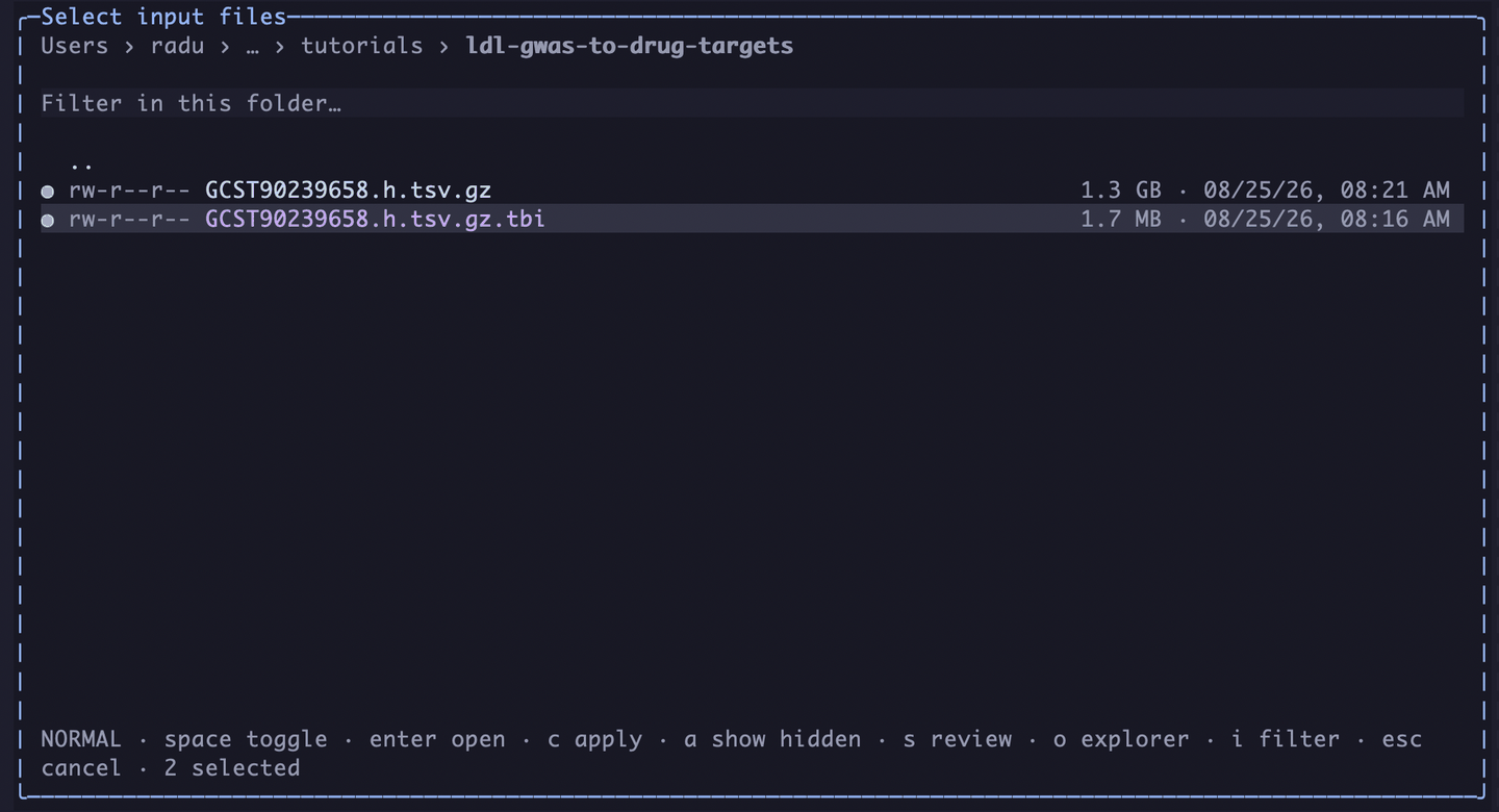
There is no accession to resolve here the way there is for a GEO series. The summary statistics come off the GWAS Catalog's FTP as two files, and inside Inflexa they are registered through the file picker: the table and its tabix index together, so any later step that wants one region rather than the whole table has the index beside it. As it turns out no step uses it on this file, because QC streams the lot in one pass, but that is not knowable at the point you register the inputs.
2. A file that won't say what it is
Same first question as every other tutorial on this site, and the answer is different in a way that matters.
what is this dataset about?
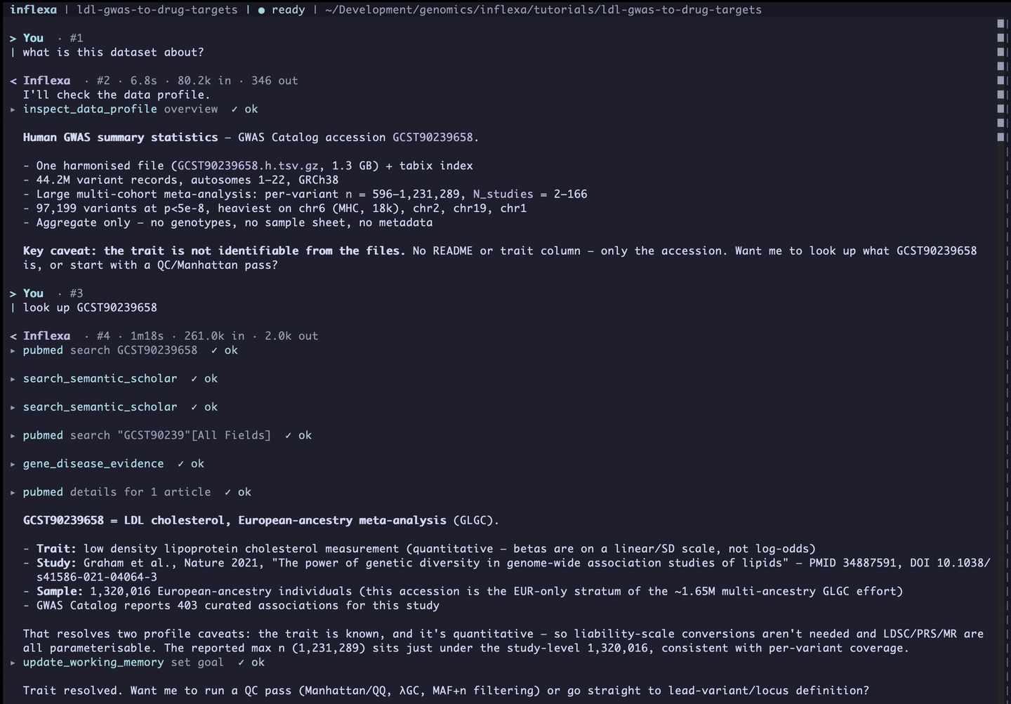
The profile comes back with the shape of the thing: 44.2 million variant records, autosomes 1 to 22, GRCh38, per-variant sample sizes running from 596 to 1,231,289 across 2 to 166 contributing studies, 97,199 variants already under the genome-wide threshold before any filtering, heaviest on chromosome 6, then 2, 19 and 1. Aggregate only. No genotypes, no sample sheet, no metadata.
Then it stops and says what it does not know: the trait is not identifiable from the files. No README or trait column, only the accession.
This is the useful moment. A model that has seen a lot of GWAS Catalog accessions could produce a confident guess about what GCST90239658 measures, and it might even be right. The profile is built from the files, so it can only report what the files contain, and what they contain does not include the trait. It asks whether to look the accession up or push on to a QC pass.
3. Looking up the accession
look up GCST90239658
Six queries, a minute and eighteen seconds: PubMed twice, Semantic Scholar twice, a gene and disease evidence lookup, then PubMed details on the one article that matched. The answer is GLGC, Graham et al., Nature 2021, PMID 34887591, LDL cholesterol, European-ancestry stratum, 1,320,016 people, and the GWAS Catalog's own count of 403 curated associations for the study.
Two facts from that lookup change what is allowed downstream. The trait is quantitative, so the betas are on a linear or standard deviation scale rather than log-odds, and no liability-scale conversion is needed anywhere. And the file's maximum per-variant n of 1,231,289 sits just under the study-level 1,320,016, which is what per-variant coverage in a meta-analysis should look like and is a quiet check that the right file is open.
The interesting part is not that the accession resolved. It is that the resolution came from a live literature query with a PMID attached rather than from the model's memory of the GWAS Catalog. On a target-evidence question that difference is the whole point, and it comes up again at the end of the run when drug status gets attached to gene names.
4. The prompt, and the constraint it found first
Here is the whole scientific request. It names three deliverables and no methods.
I want to rank the strongest loci, map them to the genes most likely responsible, and tell me which are viable LDL-lowering drug targets, including which direction a drug would have to push each one.
Before planning anything, it goes looking for reference data: gene annotation, GRCh38 builds, an LD reference panel, variant annotation, the installed reference list, and the package list in the sandbox. Then it reports the constraint rather than working around it quietly.
No LD reference panel is installed. The 1000 Genomes phasing panel for hg38 is missing, it is roughly 12.4 GB, and installing it takes over an hour. No PLINK either. So LD clumping is not available, and locus definition will have to be distance-based. GENCODE v50 and ClinVar are both installed, both on GRCh38, so gene mapping can proceed.
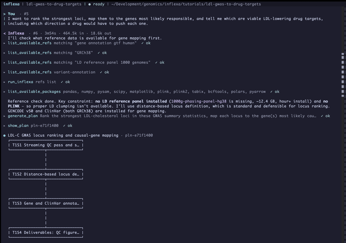
The plan is four steps: streaming QC, distance-based locus definition, GENCODE and ClinVar gene mapping, then the ranked table and figures. Before asking for approval it flags two things about itself.
- No LD clumping, and what that costs specifically. Loci will be distance-defined by greedy ±500 kb pruning, which merges genuinely independent signals. It names where: the APOE/APOC1 cluster and the LDLR region. Secondary hits will not be resolved. It offers to install the panel, then argues against it, because PLINK still would not be there afterwards.
- The drug-target verdict is not in the plan. The plan produces a ranked, direction-annotated locus table. The tractability and existing-drug assessment is a lookup against Open Targets, ChEMBL and clinical trial registries, run on top of the results rather than computed in the sandbox. That boundary is drawn before approval, and it holds all the way into the final table.
The second flag is the one worth pausing on. The prompt asked which loci are viable drug targets, and half of that question cannot be answered from the data at all. Saying so up front, rather than answering it anyway from training data and presenting the result alongside computed columns, is the difference between a table you can hand to someone and a table you have to audit first.
5. Approve, and let it run
approved
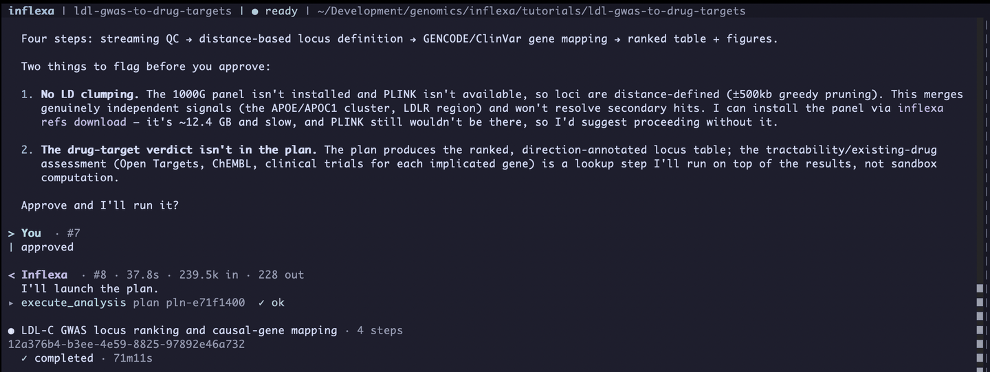
The run detaches. Each step executes in the sandbox with no network access, writing figures, tables, logs and a provenance record as it goes. Four steps, 71 minutes and 11 seconds. You can keep working in the chat pane while it does, and the run identifier is the handle for every artifact and provenance query afterwards.
6. Inflation that isn't a problem, and a p-value column that is
The QC step reads all 44,246,098 rows in a single chunked pass and never materialises the table. Two filters do all the work. Minor allele frequency below 0.01 removes 34,920,084 variants, and a sample-size floor set at half the maximum n, 615,644.5, removes a further 374,325 that pass on frequency but rest on under half the meta-analysis. What survives is 8,951,689 variants, of which 91,330 are genome-wide significant.
Note that the profile counted 97,199 significant variants and the QC step counts 91,330. The difference is the filtering, not a discrepancy, and both numbers are on the page because they answer different questions.
Then the number that makes people nervous.
λ_GC, the genomic inflation factor, is 1.4379. In a small study that reads as population stratification and a reason to stop. Here it is not, and the step makes the argument in three parts rather than asserting it. λ rescaled to an equivalent sample size of 1,000 is 1.00033, essentially 1.0, which means the inflation is proportional to N. Stratification is roughly sample-size invariant on that scale and polygenicity is not. λ is also higher among common variants, 1.5474 at MAF above 0.05, which is where more true polygenic signal sits. And the QQ curve tracks the null diagonal at low significance and departs only in the tail, which is the polygenic pattern rather than the lifted-from-the-origin pattern of confounding.
Then the sentence that makes it a QC step rather than a defence: λ is not a confounding test. The statistic that separates polygenicity from confounding is the LD score regression intercept, and computing it needs an LD reference panel, which is the thing this environment does not have. Stratification is shown to be an unnecessary explanation for the inflation. It is not excluded, and the step says so in those words.
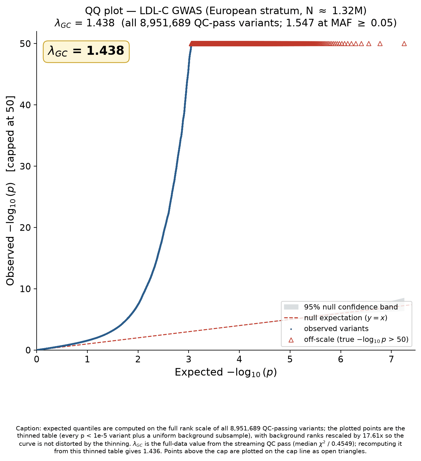
907 of the significant variants have a published p-value of exactly 0. They did not fail; they underflowed. Ranking on that column would tie the strongest signals in the file at the top and silently reorder everything below them.
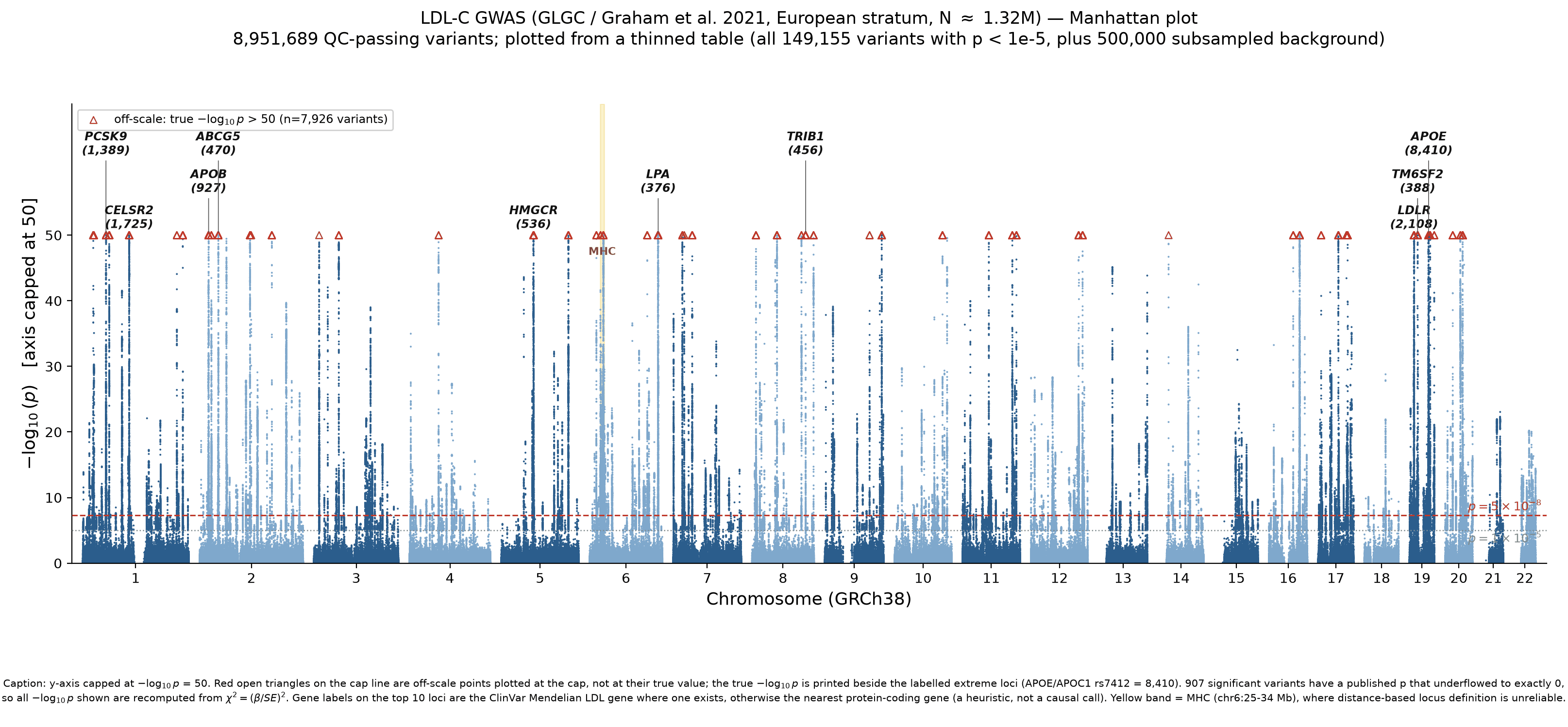
So every -log10(p) in this analysis is recomputed from chi-squared, taken as the square of beta over standard error, which stays accurate far past the point where the probability itself cannot be represented. The maximum reaches 8,410 log10 units, at rs7412 in APOE. Eleven of the top 100 leads have an underflowed published p-value, so this is not an edge case affecting obscure rows. It is the top of the table.
The recomputation was also checked against the published column where the published column is usable: median absolute discrepancy of 0.0002 log10 units across 8.95 million rows, consistent with the source p-values being rounded to about three significant figures.
Two more things in this step are worth borrowing. The harmonisation flags were enumerated rather than assumed: a census over all 44.2 million rows shows that codes 5 and 6 are 100% palindromic single-nucleotide variants, meaning strand was inferred from allele frequency. Dropping them would cost 6.36 million variants, so they are kept, but 1,315,493 retained variants carry a palindromic-inferred code and the flag travels with the artifact so a strand-sensitive downstream step can exclude them without re-reading the source. And the whole pass was executed twice and reproduced identical counts.
7. 396 loci, and what the number is not
Without LD, the fallback is distance. Take the most significant remaining variant, claim everything within 500 kb of it on the same chromosome, remove them, repeat. That produces 561 provisional loci. Merging overlapping windows brings it to 396, and those 396 partition all 91,330 significant variants exactly. 193 have a lead allele that raises LDL, 203 lower it.
The verification here is unusually direct. A deliberately naive brute-force re-derivation reproduced the window set on all 22 chromosomes with zero mismatches, the per-locus variant counts sum to exactly 91,330, and every lead is the maximum -log10(p) inside its own window with no exceptions. The estimator does what it says it does.
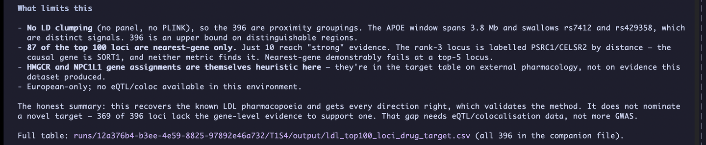
What it does not do is find independent signals, and the step is blunt about the cost. The rank-1 APOE window spans 3,824,528 bp and holds 2,694 significant variants, and it collapses rs7412 and rs429358, the two established APOE isoform signals, into one locus with only rs7412 surviving as the lead. LDLR does the same thing across 5,059,905 bp. In the other direction, 91 windows were extended past ±500 kb by merging, the largest reaching 6.56 Mb, and 30 loci rest on a single significant variant.
So 396 is an upper bound on distinguishable regions, not a count of independent associations, and it is not comparable to the count in the parent publication, which used LD-aware conditional analysis. That limitation is not left in the prose. Every row of the written table carries an ld_clumping_performed column set to false and a method note, and the file opens with a fourteen-line header stating the constraint. Anyone who opens the table in six months without reading this page still gets told.
Before any of this is used, the direction convention is checked against five variants whose direction is known outside this dataset. APOE ε2 (rs7412) lowers, PCSK9 R46L (rs11591147) lowers, APOE ε4 (rs429358) raises, the LDLR intron 1 variant rs6511720 lowers, and HMGCR rs12916 raises. All five come out right from the summary statistics alone, and the raising and lowering allele columns follow the sign of beta on all 396 loci.
That check is the licence for everything in section 11. If the harmonisation, the allele orientation or the effect scale were wrong anywhere in the chain, every directional drug call would invert without any other symptom.
8. Where nearest-gene fails, demonstrated rather than warned about
The annotation step streams an 11.2 million line GENCODE v50 GTF, filters to the 78,733 gene rows before the attribute regex runs, and loads 20,107 protein-coding genes. Every one of the 396 loci gets a nearest gene, by two metrics rather than one: distance to the nearest transcription start site, and distance to the nearest gene body.
Reporting both is the choice that makes the failure visible. The two metrics disagree at 129 loci, 32.6% of the total. One number, picked arbitrarily, would have hidden that a third of the annotation is a coin flip between two defensible answers.
Then the specific failure, at rank 3.
LOC0003 is chr1:109,274,968, lead variant rs12740374, the third-strongest signal in the genome at 1,725 log10 units. Nearest gene by transcription start site is PSRC1, at 9,139 bp. Nearest by gene body is CELSR2. The window contains 41 protein-coding genes. The causal gene at this locus is SORT1, which is in the window, and neither metric names it. The functional work that settled this showed the lead variant itself creates a C/EBP binding site that alters hepatic SORT1 expression, and SORT1 is roughly 123 kb away and the fourth-nearest protein-coding gene. No distance metric could have found it.
This is a known result, which is exactly why it belongs here. It is a positive control on the heuristic, and the heuristic fails it inside the top five. If proximity cannot name the gene at the third-strongest signal in the genome, it should not be trusted at rank 60.
Both columns in the written table are named nearest_gene_by_tss__HEURISTIC_not_causal and nearest_gene_by_body__HEURISTIC_not_causal. The warning is in the schema, where a reader loading the CSV into a dataframe six months from now will still see it.
Two more details from the top 30 give the heuristic's spread. Distances to the nearest transcription start site range from 304 bp at HNF1A to 174,266 bp at PPP1R3B, so "nearest" carries wildly different confidence locus to locus. And at rank 30 the two metrics split usefully rather than uselessly: nearest by start site is CEP112 at 22,211 bp, while nearest by gene body is APOH, a lipid gene the start-site metric misses entirely.
9. What ClinVar rescues, and what it adds as noise
The second annotation layer asks a different question. Instead of what is nearby, it asks which genes in the window carry pathogenic or likely pathogenic coding variants, which is evidence that attaches to genes rather than to positions. Across all 396 windows that returns 99,709 qualifying variants, pulled by tabix region query so the 193 MB ClinVar VCF is never scanned end to end.
Raw counts are useless as an evidence score, and the run demonstrates why before using them. 368 of 396 loci have at least one pathogenic coding variant. Only 48 have one under a lipid condition. The top ClinVar gene by count in the rank-1 APOE window is FKRP, with 227 variants, not APOE. At the ABO locus, TSC1 contributes 1,089 pathogenic coding variants and not one of them is lipid-related. Condition filtering is what turns the layer from noise into evidence.
Filtered to lipid conditions and to a Mendelian LDL gene list, 11 loci carry support. In four of those eleven, the gene ClinVar names is not the gene proximity picked:
| Rank | Lead | Nearest by TSS | ClinVar names | Lipid P/LP |
|---|---|---|---|---|
| 17 | rs598253 | USP1 | ANGPTL3 | 9 |
| 18 | rs964184 | BUD13 | APOC3 | 26 |
| 37 | rs10903129 | MACO1 | LDLRAP1 | 65 |
| 303 | rs2250781 | IFIT2 | LIPA | 90 |
Each of the four is an established Mendelian lipid gene, so none of the individual assignments is new. What the four-out-of-eleven hit rate measures is the marginal value of a cheap, entirely public evidence layer over proximity, and two of the four could not have been reached any other way without functional data. ANGPTL3 lies entirely within the intron span of DOCK7 on the opposite strand, so no distance metric reaches it. LIPA physically contains the IFIT1, IFIT2 and IFIT3 cluster, which is why the nearest-gene call came back IFIT2 at 35,981 bp.
ANGPTL3 is the one with the sharpest ending. Heterozygous loss of function carriers have substantially reduced coronary disease risk, and the gene is the target of the approved antibody evinacumab. Proximity called that locus USP1 and would have thrown it away.
ClinVar ascertainment reflects clinical testing history as much as biology. LDLR carries 4,224 pathogenic coding variants in this data because it is intensively sequenced in clinic, not because it is 4,224 times more important than a gene with one. Absence of ClinVar support at a locus is close to uninformative.
Lipid relevance here is also a keyword match on the condition field rather than an ontology mapping, and the Mendelian gene list is hand-specified. Two loci in the set are flagged lipid-relevant on one or two variants each, and the run says outright that they should not be weighted like LDLR's 1,818. The step reports its review-status breakdown for the same reason: 61,223 of the 99,709 retained variants are single-submitter assertions, and that count is carried as its own column rather than folded into a total.
10. The locus a standard filter would have deleted
Two of the 396 loci fall inside chr6:25 to 34 Mb, the extended MHC. The conventional move is to drop them, and for one of the two that instinct is completely right. LOC0033 spans 6,560,046 bp built from nine merged sub-windows, holds 10,501 significant variants and 206 protein-coding genes, and nothing about a gene list in a window that size means anything. Between them the two loci hold 12.4% of the entire significant set.
The run flags both and drops neither, with a caveat carried as a column on the rows themselves saying no causal gene should be inferred there. That decision looks like fence-sitting until you read the other locus.
LOC0032 is led by rs1800562, which is HFE C282Y, the common hereditary haemochromatosis variant. It carries a negative beta, meaning the effect allele lowers LDL, at 94.5 log10 units. Published work reports HFE variants associating with reduced LDL cholesterol in the GLGC data itself, with a mechanism running through HFE as a negative regulator of the hepatocyte LDL receptor, phenocopied in Hfe-null mice. HFE is an MHC-class-I-like iron regulatory gene sitting about 3 Mb from HLA-A, not a classical HLA gene at all.
So a blanket chr6:25 to 34 Mb exclusion, which is the standard hygiene step, would have silently deleted a mechanistically validated LDL locus while retaining nothing of value from the other one. Flag and retain, with the specific caveat attached to the specific row, lets a person adjudicate. A blanket rule that is correct on average is wrong exactly where it matters.
11. Direction is the finding, not a formality
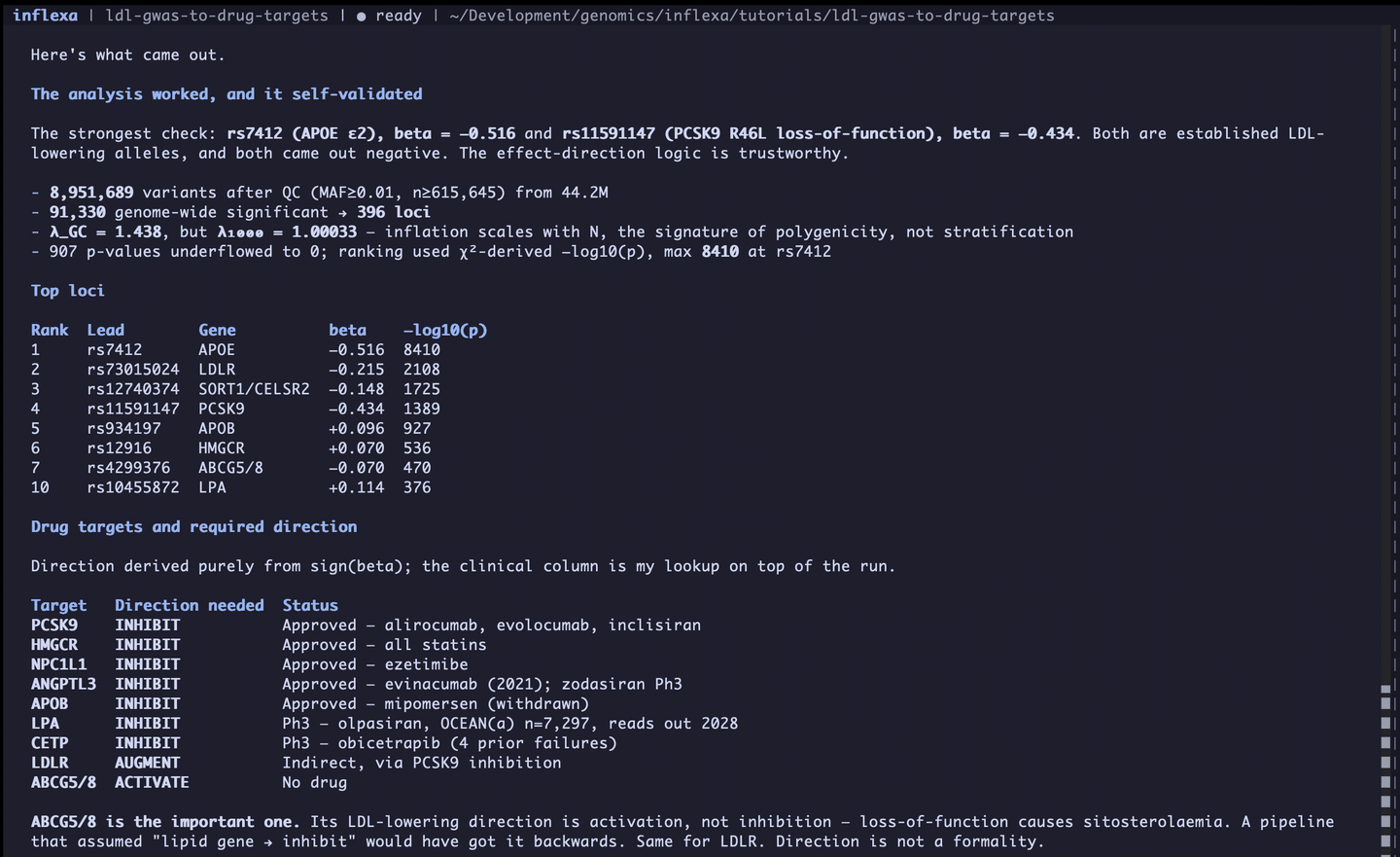
All nine canonical LDL drug targets were recovered as significant loci, and every one carries the direction established pharmacology requires. Seven of the nine are in the top ten by significance, and the furthest down the list is NPC1L1 at rank 25.
| Target | Rank | Lead | beta | Direction | Gene call |
|---|---|---|---|---|---|
| LDLR | 2 | rs73015024 | -0.215 | AUGMENT | ClinVar + Mendelian |
| PCSK9 | 4 | rs11591147 | -0.434 | INHIBIT | ClinVar + Mendelian |
| APOB | 5 | rs934197 | +0.096 | INHIBIT | ClinVar + Mendelian |
| HMGCR | 6 | rs12916 | +0.070 | INHIBIT | Nearest gene only |
| ABCG5 / ABCG8 | 7 | rs4299376 | -0.070 | ACTIVATE | ClinVar + Mendelian |
| LPA | 10 | rs10455872 | +0.114 | INHIBIT | ClinVar + Mendelian |
| ANGPTL3 | 17 | rs598253 | -0.042 | INHIBIT | ClinVar + Mendelian |
| NPC1L1 | 25 | rs17725246 | +0.043 | INHIBIT | Nearest gene only |
Eight rows, nine targets: ABCG5 and ABCG8 share a locus and are listed separately in the artifact.
ABCG5/ABCG8 is the control that proves the logic is doing something. It is a textbook lipid gene at rank 7, and its LDL-lowering direction is activation, not inhibition. The two proteins form the heterodimeric pump that exports sterols out of enterocytes and hepatocytes; biallelic loss of function causes sitosterolaemia, a sterol accumulation disease with premature atherosclerosis. Inhibiting them would raise sterol burden. A pipeline that mapped "lipid gene" to "inhibit" would have got this exactly backwards, and it is the seventh-strongest signal in the genome, not an obscure edge case.
LDLR runs the same way for a different reason. It is the rank-2 locus, and it is an augmentation target: LDLR clears LDL from plasma, loss of function causes familial hypercholesterolaemia, and the entire PCSK9 inhibitor class works by indirectly raising LDLR surface activity. Two of nine canonical targets, one of them the second-strongest signal in the genome, require pushing the target up.
Two rows in the table also carry the honest label. HMGCR and NPC1L1 are in it on nearest-gene assignments, with the ClinVar support flag reading false. They are the statin and ezetimibe targets, and everybody knows they belong, but the evidence putting them there is external pharmacology rather than anything this dataset produced, and the column says so.
The synthesis pass flagged a limit that the target table does not carry on its face. The sign of beta gives the direction of the allele's effect on LDL cholesterol. It does not give the direction of intervention on the gene product, and the two come apart wherever the mechanism is receptor clearance rather than ligand production.
Two loci in the top ten do exactly that. The LDL-lowering allele at rs6511720 increases LDLR expression, and APOE ε2 lowers LDL through a loss of receptor binding. At both, reading "lowering allele, therefore inhibit" inverts the recommendation. Getting from sign of beta to a drug direction needs a per-locus loss-or-gain-of-function annotation, which this run does not have and which is why the direction column above is right by way of external mechanism knowledge rather than by rule.
Two more top-ten rows are traps of a different kind. LPA at rank 10 looks like a target with a clean effect size, but cholesterol carried on Lp(a) particles is measured inside conventionally assayed LDL cholesterol, so the beta at that locus is substantially a measurement artifact. Published estimates put the coronary benefit of 10 mg/dL of Lp(a) lowering at 5.8% against 14.5% for the same LDL reduction, so scaling an Lp(a) target off an LDL beta overstates it by roughly two and a half fold. And TM6SF2 at rank 9 has an LDL-lowering allele that is directionally correct and carries a documented hepatic steatosis and fibrosis liability. Correct direction, invalid target.
The verdict
The two halves of a drug-target row degrade very differently when you take away the LD panel, and that is the transferable result here.
Direction of effect is carried by the sign of beta against a named effect allele. It needs no LD information at all, it was verified against five variants of known direction before being used, and it came out right at all nine canonical targets including the one where activation rather than inhibition is therapeutic. That half is solid.
Gene identity has no such anchor. The two distance metrics disagree at a third of loci, both are wrong at rank 3 in a way the literature settled fifteen years ago, and 369 of 396 loci end the run in the heuristic-only tier. The ClinVar layer is the answer to that asymmetry and it works, because pathogenic coding variants attach to genes rather than to positions, but it reaches 48 loci out of 396.
The run's own closing summary is the right one to quote: it recovers the known LDL pharmacopoeia and gets every direction right, which validates the method, and it does not nominate a novel target. 369 of 396 loci lack the gene-level evidence to support one. That gap needs eQTL and colocalisation data, not more GWAS.
That last sentence is the useful one. At N = 1.32M the data are not the limiting factor. A larger sample sharpens the association signal; it does not tell you which of 41 genes in a window the signal acts through. The honest state of the deliverable is 13 of the top 100 rows carrying orthogonal gene evidence and 87 labelled proximity-only, which is a better starting point for prioritisation than a list that hides the distinction.
If you run this yourself, those are the numbers to compare against. A run that recovers all nine canonical targets, calls ABCG5/ABCG8 as activation, and tells you that most of its own gene assignments are guesses, is working. A run that returns 396 clean target nominations is telling you something about the tool rather than about the biology.
What is still open
The report closes with three decisions it cannot make from this input. Two of them need capabilities this environment does not have.
- Whether to install an LD reference panel and clumping tooling. This replaces proximity groupings with statistically independent signals and enables the conditional analysis that would split APOE back into its two real signals. It changes the locus count. It does not, on its own, resolve a single causal gene.
- Whether to source eQTL and colocalisation data. This is the layer that moves loci off the nearest-gene heuristic, and it is the only route to a defensible novel-target nomination. It is what separates the 10 strong loci in the top 100 from the 87 heuristic ones, and it is what would have named SORT1 at rank 3.
- Whether the 296 loci below rank 100 deserve a systematic pass. Effect size and biological tractability are not the same thing as p-value. A modest beta at a well-understood gene may be more actionable than a large one in a gene desert, and rank ordering by significance does not surface that.
None of them were run. The session stopped where the evidence stopped, which is also why the write-up can be specific about what it does not know.
The full report, and the data package
This page is the walkthrough. The full report and the data package carry the rest, and they exist so that you do not have to take the write-up on trust.
The generated report
"LDL-Cholesterol GWAS: Locus Ranking, Causal-Gene Mapping, and the Direction a Drug Must Push". Every figure, every table with its data downloadable, the methods as executed, and each numeric claim linked back to the artifact and column it came from. It is the document this page was written from.
The report ships as a self-contained HTML file inside the Zenodo package below. Open it in a browser after downloading.
The data package
The scripts as they were generated and run, and every output file: the ranked top-100 table, all 396 loci in the companion CSV, the 91,330 significant variants with their locus assignments, the ClinVar variant table, and the logs with every assertion result. Enough to reproduce the run without this page, or to check any number on it.
10.5281/zenodo.22224255Your turn
The GWAS Catalog holds tens of thousands of harmonised summary statistic files, and the prompt barely changes between them:
I want to rank the strongest loci, map them to the genes most likely responsible, and tell me which are viable [your trait] drug targets, including which direction a drug would have to push each one.
Three habits from this run transfer to any of them.
Find out what reference data you have before you choose a method, because the answer changes which method is defensible rather than which one is convenient. Put a positive control where the failure would be silent: the five known-direction variants here cost nothing and were the only thing standing between a clean-looking table and a fully inverted one. And when a column is a heuristic, name it one in the schema, not in a paragraph that travels separately from the file.
If you want to start with this exact dataset, it is one accession and one index file, and the first prompt is on this page.
Run this on your own data.
Inflexa is free and open source under Apache 2.0. It runs on your machine, with the model you choose, and every result carries a record of how it was made.